How a chain of failures produced the LLM (part 1) — from the limits of maths to the geometry of meaning
The LLM as a by-product of unrelated problems: Turing on computability, Shannon on information, the perceptron, backpropagation, GPUs, and Word2Vec.
On this page
Introduction
Large language models (LLMs) like ChatGPT and Claude were not born from the goal “let us build an LLM”.
Someone trying to prove the limits of mathematics, someone trying to reduce noise on a telephone line, someone trying to fix accuracy bugs in machine translation: each solved a completely different problem, and the by-products piled up over 80 years and became the LLM.
This article follows, in order, how those unintended connections fit together. No ML or maths background is assumed.
The trigger was a Fireship YouTube video. Its compact summary of LLM history prompted me to dig deeper into “what problem each invention was actually trying to solve”, and I decided to write this.
In part 1 (this article) I cover the birth of the concept of a computer, information theory, training neural networks, and the technique of turning words into numbers. In part 2 I follow the birth of attention for handling context, Transformers, GPT-3’s scaling revolution, and the present era of alignment and efficiency.
1. What does it mean to “compute”? — Alan Turing (1936)
The problem being solved
In 1930s mathematics there was a dream:
“Every mathematical proposition should be decidable as ‘true or false’ by an algorithm.”
This was called the decision problem (Entscheidungsproblem), posed by the mathematical giant Hilbert. In short, “can mathematics be fully mechanised?”
The British mathematician Alan Turing set out to prove whether this was true.
Turing’s translation: from a maths question to a program question
Turing’s brilliant move was to translate the question into another question.
If an “algorithm that decides mathematical propositions” existed, it would have to work like this:
Keep searching for a proof → halt if a proof is found → loop forever if none is found
So “can mathematics be mechanised?” becomes the same as “can we decide whether a program halts or loops?”
Therefore, if you could prove the halting problem is unsolvable, you could prove that mechanising mathematics is impossible too. That is what Turing aimed at.
The “halting problem”: the contradiction that self-reference produces
“For any program, can we build a universal program (a decider H) that decides before running whether it halts or loops?”
The answer is No, and the way to see it is to assume the opposite. Suppose H does exist. It takes two things, a program and that program’s input, and it always answers correctly:
H(P, I) → "halts" or "loops"The shape of what goes wrong is already familiar from the liar’s paradox:
“This statement is false.” → If true, it is false. If false, it is true. Either way, a contradiction.
Turing built the same trap out of H. If H exists then so does a contrarian program D, because D is only four lines wrapped around it:
D(X): if H(X, X) == "halts": loop forever else: haltD asks H what program X does when X is given itself as input, and then does the opposite.
Now run D with D itself as its input. Its first act is to compute H(D, D), and H has to answer, because H answers for everything:
There is no third row. H’s answer is a prediction about what D does, and D reads that prediction and does the other thing. What gets falsified is not D’s behaviour but H’s verdict.
That is enough to finish it. H was supposed to be correct about every program, and D is a program it is wrong about, so H is not a correct decider. D is nothing exotic either: if H can be written at all, so can D. Decider H cannot exist in principle.
So the dream of “fully mechanising mathematics” was proven impossible.
The unintended by-product: the concept of a computer that “does everything with one machine”
What matters is not the proof’s conclusion but what the proof required.
To “prove the halting problem”, Turing first had to rigorously define “what it means to compute”. For that the Turing machine was born: an abstract model of a machine that reads and writes symbols on a tape and changes state according to rules.
Turing then noticed a decisive property of this machine. A program is itself data.
What does that mean? You can write “input data” on a Turing machine’s tape. But you can also write “the procedure for how it operates (the program)” on the same tape. So the procedure is a kind of data too. And that means you can build a universal machine that takes any program’s description as input and executes it.
This is the Universal Turing Machine (UTM).
Why this idea was revolutionary is clear compared with the world before it:
This is your laptop. The browser, games, LLM inference: the hardware does not change. Only the “data” that is the program changes.
John von Neumann read Turing’s paper and, in the 1940s, translated this concept into an actual computer design (the von Neumann architecture). Store the program in the same memory as the data: every computer today follows this design.
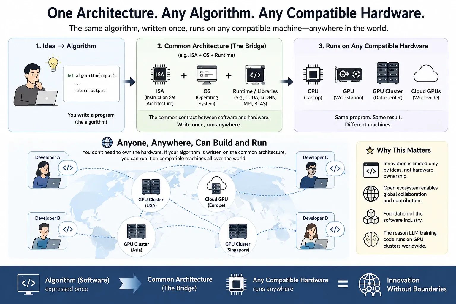
Because this design became the industry standard, something decisive happened. Any algorithm expressible on this common architecture runs on any compatible hardware. Anyone can write a program and run it on compatible machines worldwide. Without owning a dedicated machine, you can take part with only the idea of an algorithm. This is the foundation of the software industry, and the reason LLM training code runs on GPU clusters worldwide.
But the 1936 proof settled one more thing. The “limit of computability” Turing himself drew applies to LLMs too. Neither ChatGPT nor Claude can, in principle, solve the halting problem, meaning it is impossible to fully guarantee whether an arbitrary program is correct. The same paper that gave birth to the computer also defined a permanent ceiling for every AI that runs on it.
Trying to prove the limits of mathematics gave birth to the concept of a computer that does everything with one machine.
Aside: 14 years later, in 1950, Turing posed the question “can machines think?” and proposed the Turing test, which checks whether a human and a machine can be told apart. It is the conceptual ancestor of the conversational tests used to evaluate LLM capability. The highest honour in computer science is called the Turing Award (ACM Turing Award), prestigious enough to be called “the Nobel Prize of computer science”. As covered later, the pioneers of deep learning also received it.
2. Can “information” be measured mathematically? — Claude Shannon (1948)
The problem being solved
In the 1940s, Claude Shannon, a researcher at Bell Labs, had a practical worry.
“Over a noise-filled telephone line, how accurately can information be sent?”
A telephone-engineering problem, unrelated to AI or machine learning.
Why “what is information” had to be defined
Telephone engineers of the day dealt with noise intuitively: amplify the signal, improve cable quality, repeat the message. But they could not answer one fundamental question.
“On this noise-filled line, how accurately can information be sent in theory? Where is the limit?”
The reason they could not answer is simple. They could not mathematically define what the noise was breaking.
Consider it. Noise breaks the signal. So “what” part of the signal is a problem when broken?
For example, if the message “THE CAT SAT ON THE MAT” is partly garbled by noise:
- The “C” in “CAT” is lost → meaning breaks. Fatal.
- “THE” becomes “TH_” → the reader can restore it. No problem.
- The second “THE” is lost → the reader already predicts it. Information loss is small.
Here is an important discovery. Not every part of a message carries equal information. Easily predictable parts carry little information; hard-to-predict parts carry much. Noise truly does harm when it breaks the high-information parts.
So to fight noise, you first need to know “what to protect”. To know what to protect, you need to define “what information is”.
Defining “amount of information”
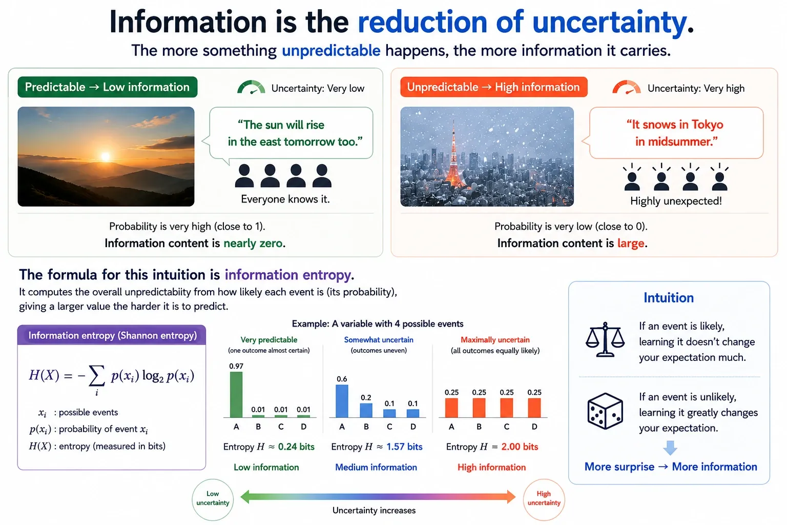
Shannon’s answer: “Information is the reduction of uncertainty. The more something unpredictable happens, the more information it carries.”
“The sun will rise in the east tomorrow too”. Everyone knows it, and the information content is nearly zero. “It snows in Tokyo in midsummer”. Unexpected, and the information content is large.
The formula for this intuition is information entropy. It “computes the overall unpredictability from how likely each event is (its probability)”, giving a larger value the harder it is to predict.
The unit of information
Incidentally, the word “bit” also appears in this era, but Shannon did not invent it himself. The concept of binary 0 and 1 goes back to Leibniz (1703), and the word “bit” was coined by his colleague John Tukey and popularised by Shannon in his paper. Shannon’s essential invention was not “0 or 1” but the mathematics of quantifying information itself.
Aside: Anthropic’s AI assistant “Claude” is widely said to be named after Claude Shannon. An AI bearing the name of Shannon, who created information theory, is a rather suggestive choice.
The engineering that Shannon’s answer unleashed
By defining information, everything became quantifiable:
- You can measure a message: compute how many bits of information it contains
- You can measure a channel: compute how many bits per second the line can carry reliably (channel capacity)
- You can design redundancy: compute how many bits to add for error correction
And the most important result is the noisy-channel coding theorem: as long as the information rate stays below the channel capacity, no matter how much noise there is, with appropriate coding you can communicate with effectively no errors.
Before Shannon, engineers thought degraded quality was unavoidable on a noisy line. Shannon proved otherwise. Noise sets a limit, but below that limit perfect reliability is achievable, given the right coding.
The connection to compression: low-information parts can be discarded
Shannon’s definition of information produced another revolution: data compression.
By the source coding theorem, the theoretical minimum size to which a message can be compressed equals its entropy (information content). That is:
- “AAAAAAAAAA”: completely predictable, entropy near zero → compressible to nearly zero
- Random noise: completely unpredictable, maximum entropy → not compressible
- Natural language: in between, many patterns → highly compressible
JPEG, MP3 and ZIP files are all this principle. Remove the easily predicted (low-information) parts and keep the hard-to-predict (high-information) parts. On decompression, restore the parts predictable from context.
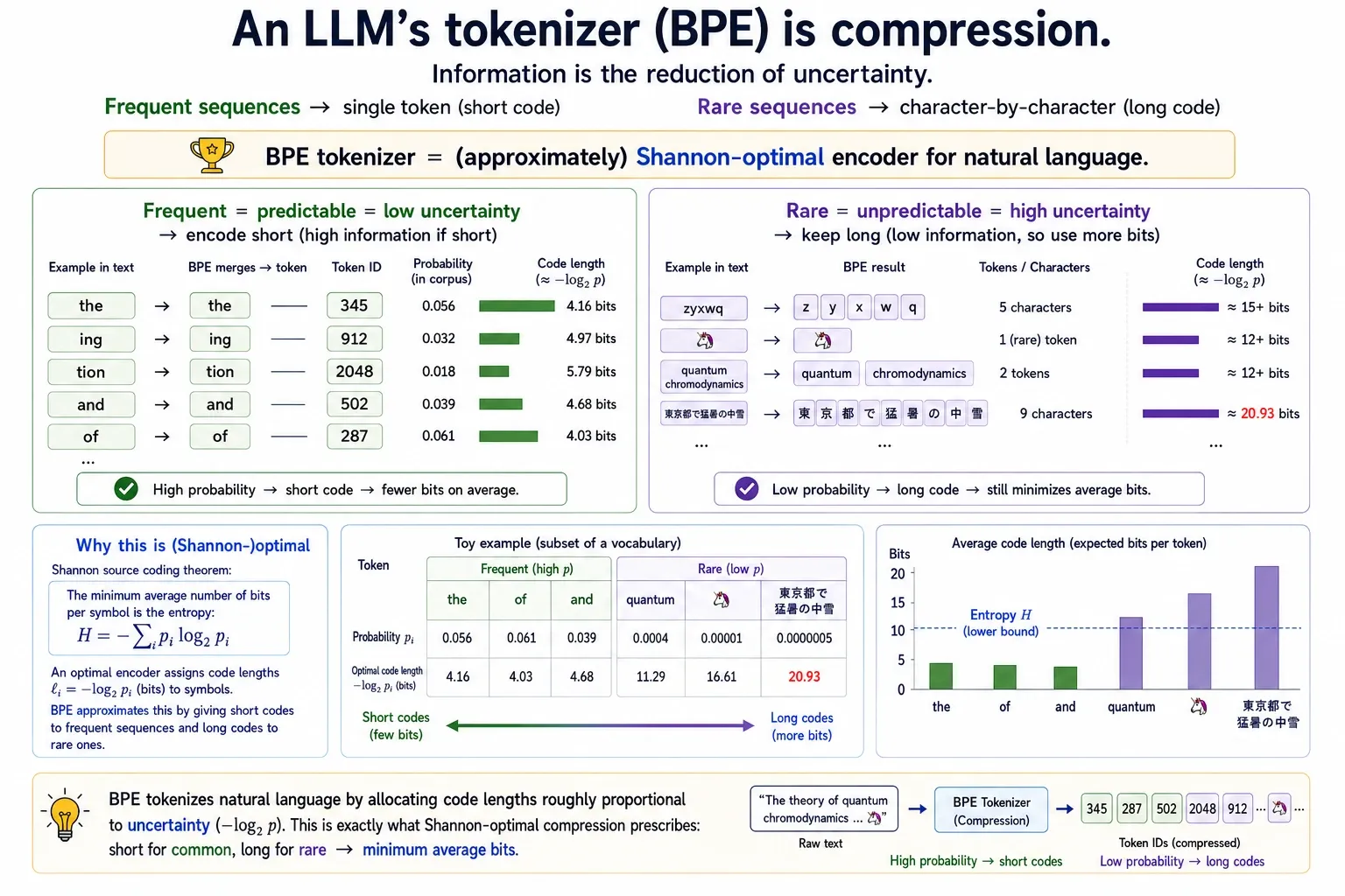
An LLM’s tokenizer (BPE, or Byte Pair Encoding) is compression in this sense too. Frequent sequences (“the”, “ing”, “tion”) become a single token, and rare sequences stay character-by-character. The tokenizer is literally a Shannon-optimal encoder for natural language.
The connection to LLMs: from training to inference
Training: cross-entropy loss
The core question when training an LLM is “how accurately can the model predict the next word?”
The metric used to measure this “accuracy of prediction” is cross-entropy loss, derived directly from Shannon’s entropy.
loss = -(sum of correct-answer probability × log(model's predicted probability))When an LLM learns, the model relentlessly tries to make this number smaller. In other words, reducing the “surprise” at the next token is the entire purpose of training. Shannon’s “information = reduction of uncertainty” is directly the learning objective.
Inference: temperature is the entropy knob
Shannon’s notion of “surprise” also connects directly to controlling LLM output. The temperature parameter is a knob that directly manipulates the entropy of the output distribution.
P(token) = softmax(logit / temperature)| Temperature | Effect on the distribution | Shannon entropy |
|---|---|---|
| → 0 | Concentrates on the highest-probability token | Entropy → 0 (zero surprise) |
| = 1 | The model’s natural distribution | Natural entropy |
| > 1 | Distribution flattens, all tokens more equal | Entropy rises (surprise increases) |
Low temperature = always pick the most predictable (low-information) token. High temperature = sample from a higher-entropy distribution = creative but possibly less consistent.
When you raise the temperature to “write more creatively”, you are literally raising the Shannon entropy of the output.
The whole connection
One mathematical framework applies to every layer of building and running an LLM. Shannon’s mathematics, which wanted to reduce telephone-line noise, has become 80 years later both the LLM’s “definition of smartness” and its “creativity adjustment knob”.
3. Can machines learn? — optimism, setback, revival
The age of optimism: the perceptron (1958)
The first demonstration that “a machine can learn” was Frank Rosenblatt’s perceptron.
The mechanism is simple. The simplest neural network is a circuit of just one “neuron”.
- Take several inputs (numbers)
- Multiply each by a “weight” and add them
- If the sum exceeds a threshold, output “Yes (1)”; otherwise “No (0)”
Look at a concrete example. A perceptron that decides “is this email spam?”:
inputs:  x1 = contains "free prize"? (1 or 0)  x2 = from a known contact? (1 or 0)  x3 = has an attachment? (1 or 0)
learned weights:  w1 = +0.9 (strong spam signal)  w2 = -0.8 (strong non-spam signal)  w3 = +0.3 (weak spam signal)
score = (1)(0.9) + (0)(-0.8) + (1)(0.3) = 1.2threshold = 0.51.2 > 0.5 → "spam"
“Learning” is adjusting these weights. Start with random weights, check against the answers, and correct the weights little by little. Repeat thousands of times and the weights converge to appropriate values.
Before the perceptron, every program ran on rules handwritten by humans. The perceptron demonstrated the revolutionary concept that a machine finds its own rules from data.
The New York Times reported: “the Navy revealed the embryo of a machine that can walk, talk, see, write, and reproduce itself”. An air of optimism prevailed.
Setback: the first AI winter (1969)
Marvin Minsky and Seymour Papert threw cold water on it.
The perceptron has a mathematical limit.
A question may arise here. “As Turing proved in 1936, a universal Turing machine can perform any computation. Why would something like XOR be a problem?”
The answer is that Turing’s universality and the perceptron’s learning are completely different abilities.
- Turing’s universality: if a human writes the right program, any computation is possible. XOR? A single
ifline. - The perceptron’s promise: the machine discovers the rules itself from data. Humans do not write the rules.
What XOR destroyed was not “computational power” but the “learning mechanism” itself.
Look concretely. XOR (exclusive OR) is the simple rule “0 if both inputs are 1 or both are 0, and 1 if only one is 1”. Plotted on a 2D plane:
The perceptron tries to separate Yes and No with a single straight line. But look at the figure above: separating ● and ○ with one straight line is impossible. However you draw the line, they always mix.
If that were all, “so XOR is a special case” might suffice. But what Minsky and Papert proved was not just about XOR. They showed that an entire class of problems requiring non-linear decision boundaries was impossible for the perceptron: parity (odd/even), symmetry detection, connectivity, and more. XOR is only the simplest, most embarrassing counterexample.
And the reason this was devastating is the gap between expectation and reality. The media reported “a machine that walks and talks”. Mathematicians proved that machine cannot even learn XOR. The funders’ conclusion: “neural networks = a dead end”. This triggered the first AI winter. Research funding froze and many neural-network researchers lost their jobs.
But their book carried one line of note:
“A multi-layer network might solve this problem. But how to train it is unknown.”
This “but” defined the research question for the next 17 years.
Revival: backpropagation (1986)
The “but” was solved by backpropagation (error back-propagation) from Rumelhart, Hinton, and Williams.
A multi-layer network is several perceptrons connected together. Each perceptron has its own weights, grouped into layers.
In this figure the middle Layer 2 is called the hidden layer. “Hidden” does not mean it hides anything. The input layer is where the user hands over data, the output layer is where the user receives the result. Both are “visible” to the user. The middle layer, by contrast, is an internal workspace the user never touches directly. It is “hidden” because it is invisible from outside.
Why “deep” learning?
When layers increase, it is these hidden layers that increase. There is always one input layer and one output layer. How many hidden layers you stack between them is “the depth of the network”, and that is the meaning of “deep” in “deep learning”. This “hidden” concept reappears in chapter 5, so keep it in mind.
The learning flow is intuitive:
- Initialise all weights to random values (if not random, every neuron learns the same thing)
- Feed in data and produce a prediction through all layers (“this image is a cat”)
- Check against the answer and compute how wrong it was
- Trace, backwards from output to input, “which weights contributed to this error”
- Adjust each weight slightly by its contribution (weights are overwritten; no snapshot remains)
- Repeat this millions of times
How is “which weight contributed how much to the error” computed?
Only the final output knows the correct answer. Nobody knows what the intermediate layers “should correctly output”. There is no correct answer for “Layer 1’s correct edge-detection result for a cat image”.
So the error signal is propagated backwards from the output. Using the chain rule of calculus, each layer’s responsibility is computed in turn: if A affects B and B affects C, then A’s effect on C is the product of the two effects.
The error propagates backwards. Hence backpropagation.
It was shown that multi-layer networks can be trained this way, solving the problem Minsky and colleagues called “unknown”.
Why does going multi-layer solve it? The core is the difference between linear and non-linear. A perceptron (single layer) can draw only one straight line. That is the limit of linear. In a multi-layer network, each layer draws its own straight line, and combining them makes curved and complex decision boundaries. That is non-linear.
The more layers, the more complex the decision boundary. This is the foundation of deep learning.
But there was a large wall between theory and practice. Training multi-layer networks needs enormous computation, and 1980s–90s hardware could not run training at practical speed.
Breaking the speed wall: the arrival of GPUs (2012)
Even with backpropagation established, multi-layer networks stayed far from practical for a while. Not enough data. Computation too slow.
In 2012, the situation changed at ImageNet (a contest to classify over a million images into 1,000 categories). A model called AlexNet posted an overwhelming result. Against the second-place error rate of 26.2%, AlexNet scored 15.3%, a gap of about 11 points. In machine learning a 1–2 point year-on-year improvement is normal, so 11 points was an understatement even called “crushing”. Many computer-vision researchers switched to deep learning en masse the next year, and the industry’s common sense was rewritten.
What AlexNet used was the GPU (graphics chip). Why was the GPU so effective? Training until then was done on CPUs, but CPUs and GPUs differ fundamentally in design philosophy.
A CPU has a few high-performance cores (4–16) and is designed to handle complex tasks sequentially. A GPU has thousands of simple cores (over 4,000) and is designed to run many simple computations simultaneously.
Training a neural network is, for the most part, matrix multiplication: the simple repetition of multiplying thousands of weights by thousands of inputs and summing. And each multiplication is independent; the result of w3×x3 need not wait for the result of w1×x1.
Training AlexNet would have taken weeks to months on a CPU but finished in days on a GPU. Same maths, same result, just massively parallelised. The GPU broke the training-speed wall and proved that the combination “GPU + large data + multi-layer network” works at a practical level.
But AlexNet was an 8-layer network. “Deeper (more layers) should be smarter”, but trying to deepen the layers raises another wall.
Aside: one of AlexNet’s authors, Geoffrey Hinton, is also named on the 1986 backpropagation paper. Across the AI winter, the same person led deep learning’s revival 26 years later. Hinton received the Turing Award in 2018 alongside Yann LeCun and Yoshua Bengio, and the three together are called “the fathers of deep learning”.
Aside: NVIDIA, which made the GPUs, was originally a gaming-graphics company. 3D rendering in games is also “running the same computation in parallel over a huge number of pixels”, which is structurally the same as a neural network’s matrix operations. The AI boom made NVIDIA one of the most valuable companies in the world. A gaming chip becoming the optimal tool for AI training is another of the “unintended connections” this article has followed.
Deeper still: overcoming vanishing gradients (2010s)
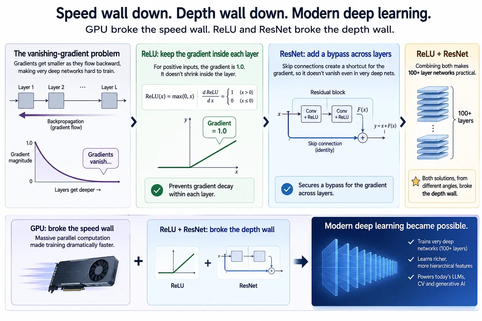
Even after GPUs solved the speed problem, deepening the network itself had another wall: the vanishing gradient problem.
As seen with backpropagation, the only scoring point is the final output. The error signal can only travel backwards up the layers. And each time it passes a layer, the signal shrinks by multiplication. Each multiplication’s coefficient is typically below 1 (e.g. 0.3), so repeatedly multiplying small numbers rapidly approaches zero.
3 layers: 0.3 × 0.3 × 0.3 = 0.027 ← small but usable10 layers: 0.3^10 ≈ 0.000006 ← nearly zero50 layers: 0.3^50 ≈ 0.00000000000000000000000... ← effectively zeroThe closer to the final layer, the stronger the feedback; the earlier the layer, the more the feedback vanishes:
This is like a building’s foundation being broken but unfixable. Layer 1 should learn basic features (edges, simple patterns), but feedback does not reach it, so it cannot learn. With the foundation left nonsense, nothing stacked on top means anything.
This wall was overcome in stages by a combination of techniques.
Why the signal was shrinking “×0.3”: the sigmoid activation function
I said each layer’s multiplication coefficient is below 1, like “0.3”. Where does this coefficient come from? The answer is the activation function, the function by which each neuron transforms its output.
Long in use was the sigmoid. The sigmoid was designed to mimic biological neurons. Real neurons are not simple on/off; they activate smoothly according to stimulus strength. The sigmoid is a smooth S-curve that reproduces this, converting any input to the range 0–1.
But in backpropagation, each layer’s “responsibility coefficient” is determined by the slope (gradient) of this activation function. The sigmoid’s slope is at most about 0.25, usually less.
Biological plausibility and mathematical elegance: the very reasons the sigmoid was thought “clever” were what killed the gradient. Its strength was its weakness.
ReLU: why “crude” won
ReLU (Rectified Linear Unit) is astonishingly simple. “Pass through if positive, zero if negative”. That is all. Mathematicians at first dismissed it. Too crude. It has a non-differentiable point. Nothing like a neuron.
But ReLU’s slope for positive values is exactly 1.0. Not 0.25, not 0.1, but 1.
ReLU does not “amplify” the signal. It merely stopped killing it. The sigmoid actively compressed the signal at each layer. ReLU passes it through.
In the 1980s networks had only 2–3 layers, so the sigmoid’s problem never surfaced. Only when layers deepened did the hidden cost of the “clever design” become fatal. At scale, the crudeness that preserves the signal beats the elegance that breaks it.
But the sigmoid was not “wrong”. It was right, but could not withstand scale. Like training wheels on a bicycle: the right design for a beginner, an obstacle for a racer. In fact the sigmoid is still used for specific purposes: Yes/No classification in the output layer (where a 0–1 probability is needed) and gate control inside memory cells. But in the hidden layers of a deep network, ReLU is now standard.
Residual connections (ResNet, 2015): another solution
Where ReLU curbed each layer’s signal decay, residual connections (ResNet) attacked vanishing gradients from a completely different angle.
In an ordinary network, each layer is required to “take an input and produce a complete output”. With a residual connection, the input passes through a shortcut path and is added directly to the output.
What does this change? The layer’s job changes fundamentally. The layer’s role changes from “produce a complete output” to “learn a small correction (residual) to the input”. Hence the name residual connection.
Think of a familiar example. To weigh a dog too light for the scale, hold the dog, step on the scale together, and subtract your own weight. Because you have a known baseline (your own weight, the input), the small difference (the dog, the residual) can be measured accurately. A residual connection is the same: by keeping the input as a baseline, the small correction the layer must learn becomes detectable.
And for the gradient there is a decisive difference too. In backpropagation, the gradient flows through both paths:
Even if the gradient shrinks to 0.001 on the layer path, the shortcut path adds 1.0. The total is about 1.001. The shortcut works as insurance, and the signal does not die. And because the gradient flows on the layer path too, the layer itself can still learn, because the feedback does not vanish.
What if the layer finds no useful correction? Output 0. Output = 0 + input = the input passes through unchanged. Because a layer has the option of “doing nothing”, adding deep layers does not degrade performance.
ResNet trained a 152-layer network successfully with this mechanism and won ImageNet 2015.
ReLU and ResNet: different approaches, the same goal
ReLU and ResNet are solutions from different angles to the same vanishing-gradient problem. ReLU prevents gradient decay inside each layer (keeping the coefficient at 1.0); ResNet secures a bypass for the gradient across layers. In modern deep learning, combining both made networks of over 100 layers practical.
The GPU broke the speed wall, and ReLU and ResNet broke the depth wall. With both the speed and depth walls down, modern deep learning became possible.
4. What does it mean to turn words into numbers? — the geometry of meaning
Computers handle only numbers
The story so far has been “how to make learning accurate”. And every success so far handled data that was numbers from the start. Images are pixel values (each pixel a 0–255 colour value). Audio is waveform values. Stock prices, temperatures, sensor data: all numbers from the start. You can feed them straight into a neural network.
But words are not numbers. “Cat”, “economy”, “beautiful”: these are symbols and cannot be fed as-is into a neural network’s matrix computation. To build an LLM, you first had to solve the fundamental problem “how do we convert words into numbers?”
The simplest method: assign numbers, “cat = 1, dog = 2, sky = 3…”. But this leaves no semantic relationship between “cat” and “dog”. The information “cat and dog are similar”, “cat and spaceship are far apart” is not in the numbers.
Word2Vec: meaning as coordinates in space (2013)
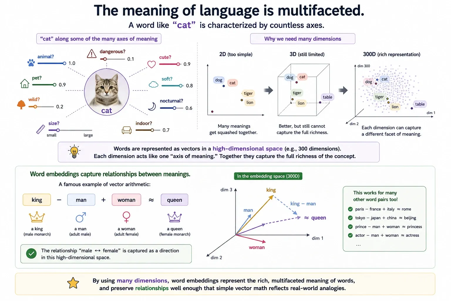
The idea Google’s Mikolov and colleagues showed: represent a word as “coordinates (a vector)” in a high-dimensional space.
What does “high-dimensional” mean? The maps we use daily are 2D (east-west, north-south); inside a building, 3D (+ up-down). Word2Vec represents one word as 300-dimensional coordinates. Humans cannot picture a 300-dimensional space, but mathematically you can compute distance and direction just as in 2D or 3D.
Why 300 dimensions? Because the meaning of language is multifaceted. The word “cat” is characterised by countless axes: “animal?”, “pet?”, “size?”, “dangerous?”, “cute?”. Two or three dimensions cannot express this rich range of meaning. With 300 dimensions, each dimension can capture a different facet of meaning.
The training method is simple. Learn so that “words appearing in similar contexts get close coordinates”. “Cat” and “dog” are both used in contexts like “pet”, “food”, “walk”, so their coordinates become close.
The resulting “map of meaning” had a surprising property:
coordinates of "king" − coordinates of "man" + coordinates of "woman" ≈ coordinates of "queen"You can do arithmetic on meaning. Language became mathematics.
Aside: the idea that “meaning lies in relationships” had a precursor. In 1998, Stanford graduate students Larry Page and Sergey Brin proposed PageRank in the paper “The Anatomy of a Large-Scale Hypertextual Web Search Engine”. Search engines of the day ranked by keyword frequency within a page, but PageRank measured importance by how much a page was linked from other pages, the structural relationships of the web. The view that “the surrounding relationships express the essence more than the content itself” is remarkably similar to Word2Vec’s “a word’s meaning is determined by its surrounding context (co-occurring words)”. And the Google born from PageRank later founded Google Brain and produced the 2017 “Attention Is All You Need” (Transformer) paper. A search-engine company invented the core architecture of the LLM. Another “unintended connection”.
How do you measure “close”? — cosine similarity
I said “cat and dog are close”, “cat and spaceship are far”, but what does “close” mean in a 300-dimensional space?
Intuitively you want to use the distance between two points (Euclidean distance). But in high-dimensional space, direction captures semantic similarity better than distance.
See the reason with a concrete example. Suppose there is a long document and a short document about “cat”.
Both are “documents written about cats”, yet measured by distance they are judged “far”. Measured by direction they are “the same”, and that is correct.
Cosine similarity measures how much two vectors point in the same direction.
The scale runs from 1.0 for exactly the same direction, through 0.0 for a right angle, to −1.0 for the exact opposite. The figure above carries both the scale and a worked example.
This is the foundation of today’s RAG (retrieval-augmented generation) and semantic search. Vectorise the user’s question, compute cosine similarity against the vectors of documents in a database, and retrieve the document closest in direction. The idea “measure meaning by direction”, which began with Word2Vec, is now the search engine of AI applications.
This technique is called Embedding.
Why Embedding is indispensable to an LLM
Embedding matters not only for RAG and search. It is the very entrance through which an LLM processes language.
An LLM’s interior is a neural network, a chain of matrix multiplications. Matrix multiplication needs vectors of numbers. You cannot put the string “cat” straight into a neural network.
Without Embedding, an LLM cannot even receive input. The technique Word2Vec established, “convert words into meaningful vectors”, is built into the LLM’s literal entrance: its first layer.
We have now solved “how to turn words into numbers”. But the next problem waits. Converting words to vectors alone loses the order of the words (context). “The dog chased the cat” and “the cat chased the dog” have the same word vectors, but opposite meanings.
How do you handle context? That question is the theme of the next chapter. And the first to tackle it seriously were researchers in machine translation.
Summary
Part 1 followed the birth of the computer through Word2Vec, and the through-line was that each invention was solving a completely different problem:
- Turing (1936): trying to prove the limits of mathematics gave birth to the concept of the universal computer, and to a permanent ceiling that applies to LLMs too.
- Shannon (1948): defining “information = the reduction of uncertainty” to fight telephone-line noise became the LLM’s cross-entropy training loss and its temperature knob.
- The perceptron to backpropagation (1958–1986): XOR triggered the first AI winter, and the “multi-layer but how to train it” question was answered by propagating error backwards.
- GPUs and ReLU/ResNet (2012–2015): breaking the speed wall and the depth wall together made modern deep learning practical.
- Word2Vec (2013): representing words as coordinates in space turned language into mathematics and became the LLM’s entrance, the Embedding layer.
The next problem is context: converting words to vectors loses their order, and “the dog chased the cat” and “the cat chased the dog” become indistinguishable. Part 2 picks up there, following the birth of attention, the Transformer, GPT-3’s scaling revolution, and the present era of alignment and efficiency. That is the second half of how the LLM was completed “without being designed”.